Classification of Chest X-Rays Using Tensorflow 2
This is the first of a two part series showing how TensorFlow can be used to create models for classifying medical images. This article shows the generation and evaluation of the model. Part two will cover the application of SHAP's GradientExplainer.
Deep Learning is a branch of machine learning that uses special computer simulations, called neural networks, to "learn" about patterns and data without being explicitly programmed. It has already had a significant impact on multiple science fields and led to improvements in speech and image recognition, fraud detection, financial analysis, and many other areas.
Programs created through Deep Learning techniques can already beat humans at complex games such as Go and StarCraft; and surpass radiologists ability to diagnose breast cancer, eye disease, and other ailments; and its influence is only beginning to be felt.
No other field will be impacted more than healthcare and biomedical science. Healthcare is a data-rich field discipline, and there is an enormous amount of untapped information to drive innovations.
One of the simplest places to start is image classification. In this post, we will be looking at the methods and tools used to classify X-Ray images into one of two categories: normal or pneumonia.
Pneumonia is an infection that inflames the air sacs in one or both lungs. It kills more children younger than five years old each year more than any other infectious disease, such as HIV infection, malaria, or tuberculosis. Diagnosis is often based on symptoms and physical examination. Chest X-rays may help confirm the diagnosis.
To do this, we will use a Convolutional Neural Network on the Tensorflow/Keras platform. For the dataset, a 150x150 standardized dataset in zip format was created containing chest x-rays from this Kaggle page. You can download it here.
To begin, let's load in our libraries:
import os
import cv2
import numpy as np
import tensorflow as tf

import matplotlib.pyplot as plt
import seaborn as sns

from sklearn.metrics import classification_report, confusion_matrix
First download then decompress the dataset. We're going to assume that it was extracted into a folder called 150x150.
Using opencv, load all of the train, test, and validation files into memory:
BASE = '150x150'
classes = ['normal', 'pneumonia']
num_classes = len(classes)

def load_data(variety):
    result = {}
    for _class in classes:
        result[_class] = []
        path = os.path.join(BASE, variety, _class)
        for file in os.listdir(path):
            img = cv2.imread(os.path.join(path, file), cv2.IMREAD_GRAYSCALE)
            result[_class].append(img)
    return result

train = load_data('train')
test = load_data('test')
val = load_data('val')
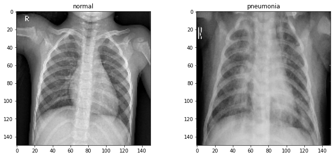
All of the XRays have been scaled so that they're all 150 by 150 pixels in size. We can verify this by viewing a random pair:
fig, axs = plt.subplots(1, 2, figsize=(12, 5))
for ax, label in zip(axs, classes):
    ax.imshow(train[label][3], cmap='gray')
    ax.set_title(label)
plt.show()
Let's take a look at the distribution of data labels:
sns.barplot(classes, [len(train['normal']), len(train['pneumonia'])])
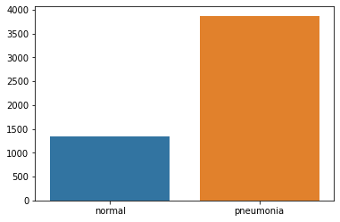
The data is unbalanced in favor of pneumonia images. To fix this, we will need to do some data augmentation.
Let's first normalize the images and create our training, testing, and validation sets:
size = 150
X_train, y_train = [], []
X_test, y_test = [], []
X_val, y_val = [], []

for k, v in train.items():
    X_train.extend(v)
    y_train.extend([classes.index(k) for i in v])

for k, v in test.items():
    X_test.extend(v)
    y_test.extend([classes.index(k) for i in v])

for k, v in val.items():
    X_val.extend(v)
    y_val.extend([classes.index(k) for i in v])

# Normalize "color" of the images
X_train = np.array(X_train) / 255
X_val = np.array(X_val) / 255
X_test = np.array(X_test) / 255

# resize data for deep learning
X_train = X_train.reshape(-1, size, size, 1)
y_train = np.array(y_train)
X_val = X_val.reshape(-1, size, size, 1)
y_val = np.array(y_val)
X_test = X_test.reshape(-1, size, size, 1)
y_test = np.array(y_test)
Now we apply the data augmentation techniques to prevent overfitting and handling the imbalance in dataset. This approach is taken from: https://www.kaggle.com/madz2000/pneumonia-detection-using-cnn-92-6-accuracy
datagen = tf.keras.preprocessing.image.ImageDataGenerator(
        featurewise_center=False,  # set input mean to 0 over the dataset
        samplewise_center=False,  # set each sample mean to 0
        featurewise_std_normalization=False,  # divide inputs by std of the dataset
        samplewise_std_normalization=False,  # divide each input by its std
        zca_whitening=False,  # apply ZCA whitening
        rotation_range = 30,  # randomly rotate images in the range (degrees, 0 to 180)
        zoom_range = 0.2, # Randomly zoom image
        width_shift_range=0.1,  # randomly shift images horizontally (fraction of total width)
        height_shift_range=0.1,  # randomly shift images vertically (fraction of total height)
        horizontal_flip = True,  # randomly flip images
        vertical_flip=False)  # randomly flip images

datagen.fit(X_train)
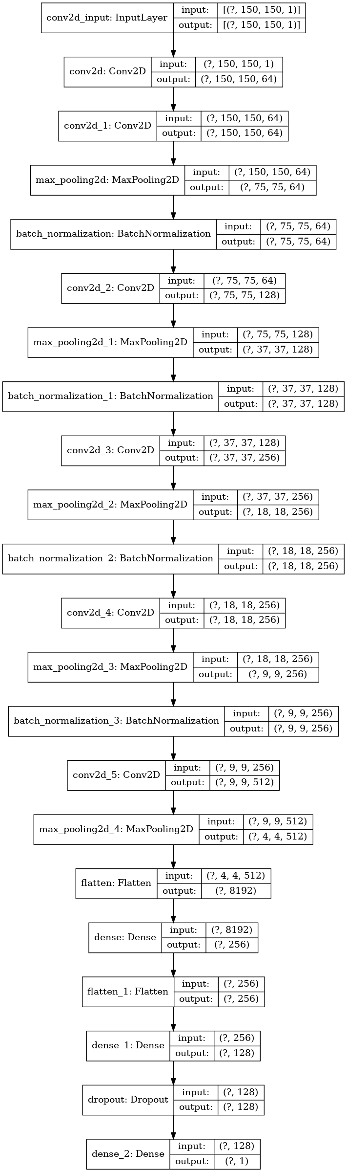
Let's assemble our model. This is a custom model structure that is loosely based off of VGG16:
model = tf.keras.models.Sequential()

# Block 1
model.add(tf.keras.layers.Conv2D(64, (3,3), padding='same', activation='relu', input_shape=(size, size, 1)))
model.add(tf.keras.layers.Conv2D(64, (3,3), padding='same', activation='relu'))
model.add(tf.keras.layers.MaxPooling2D((2, 2), strides=(2, 2)))

# Block 2
model.add(tf.keras.layers.BatchNormalization())
model.add(tf.keras.layers.Conv2D(128, (3,3), padding='same', activation='relu'))
model.add(tf.keras.layers.MaxPooling2D((2, 2), strides=(2, 2)))

# Block 3
model.add(tf.keras.layers.BatchNormalization())
model.add(tf.keras.layers.Conv2D(256, (3,3), padding='same', activation='relu'))
model.add(tf.keras.layers.MaxPooling2D((2, 2), strides=(2, 2)))

# Block 4
model.add(tf.keras.layers.BatchNormalization())
model.add(tf.keras.layers.Conv2D(256, (3,3), padding='same', activation='relu'))
model.add(tf.keras.layers.MaxPooling2D((2, 2), strides=(2, 2)))

# Block 5
model.add(tf.keras.layers.BatchNormalization())
model.add(tf.keras.layers.Conv2D(512, (3,3), padding='same', activation='relu'))
model.add(tf.keras.layers.MaxPooling2D((2, 2), strides=(2, 2)))

# Classification block
model.add(tf.keras.layers.Flatten())
model.add(tf.keras.layers.Dense(units=256, activation='relu'))
model.add(tf.keras.layers.Flatten())
model.add(tf.keras.layers.Dense(units=128, activation='relu'))
model.add(tf.keras.layers.Dropout(0.2))
model.add(tf.keras.layers.Dense(units=1, activation='sigmoid'))

# Compile
model.compile(optimizer="rmsprop", loss='binary_crossentropy', metrics=['accuracy'])
We can use the Keras plot_model utility to visualize this model:
tf.keras.utils.plot_model(model, show_shapes=True)
Create a callback that reduces the Learning Rate:
learning_rate_reduction = tf.keras.callbacks.ReduceLROnPlateau(
    monitor='val_accuracy',
    patience=2,
    verbose=1,
    factor=0.3,
    min_lr=0.000001
)
Now we can train the model. Make sure to include the datagen function and Learning Rate Reduction callback:
history = model.fit(
    datagen.flow(X_train, y_train, batch_size=32, shuffle=True),
    epochs=12,
    validation_data=datagen.flow(X_val, y_val),
    callbacks=[learning_rate_reduction]
)
Epoch 1/12
  2/163 [..............................] - ETA: 8s - loss: 1.8002 - accuracy: 0.6562WARNING:tensorflow:Callbacks method `on_train_batch_end` is slow compared to the batch time (batch time: 0.0391s vs `on_train_batch_end` time: 0.0633s). Check your callbacks.
163/163 [==============================] - 19s 115ms/step - loss: 1.1303 - accuracy: 0.7821 - val_loss: 9.6586 - val_accuracy: 0.5000
Epoch 2/12
163/163 [==============================] - 17s 103ms/step - loss: 0.3089 - accuracy: 0.8836 - val_loss: 10.4589 - val_accuracy: 0.5000
Epoch 3/12
163/163 [==============================] - 17s 103ms/step - loss: 0.2448 - accuracy: 0.9083 - val_loss: 2.4090 - val_accuracy: 0.5625
Epoch 4/12
163/163 [==============================] - 17s 102ms/step - loss: 0.1979 - accuracy: 0.9260 - val_loss: 0.4715 - val_accuracy: 0.6875
Epoch 5/12
163/163 [==============================] - 17s 102ms/step - loss: 0.1932 - accuracy: 0.9311 - val_loss: 0.2192 - val_accuracy: 0.9375
Epoch 6/12
163/163 [==============================] - 17s 102ms/step - loss: 0.1908 - accuracy: 0.9388 - val_loss: 4.2847 - val_accuracy: 0.5625
Epoch 7/12
163/163 [==============================] - ETA: 0s - loss: 0.1694 - accuracy: 0.9471
Epoch 00007: ReduceLROnPlateau reducing learning rate to 0.0003000000142492354.
163/163 [==============================] - 17s 103ms/step - loss: 0.1694 - accuracy: 0.9471 - val_loss: 0.4556 - val_accuracy: 0.8125
Epoch 8/12
163/163 [==============================] - 17s 103ms/step - loss: 0.1221 - accuracy: 0.9563 - val_loss: 4.9089 - val_accuracy: 0.5000
Epoch 9/12
163/163 [==============================] - ETA: 0s - loss: 0.1103 - accuracy: 0.9614
Epoch 00009: ReduceLROnPlateau reducing learning rate to 9.000000427477062e-05.
163/163 [==============================] - 17s 103ms/step - loss: 0.1103 - accuracy: 0.9614 - val_loss: 0.8160 - val_accuracy: 0.6250
Epoch 10/12
163/163 [==============================] - 17s 103ms/step - loss: 0.1104 - accuracy: 0.9641 - val_loss: 0.8423 - val_accuracy: 0.6250
Epoch 11/12
163/163 [==============================] - ETA: 0s - loss: 0.1043 - accuracy: 0.9632
Epoch 00011: ReduceLROnPlateau reducing learning rate to 2.700000040931627e-05.
163/163 [==============================] - 17s 103ms/step - loss: 0.1043 - accuracy: 0.9632 - val_loss: 1.1281 - val_accuracy: 0.6250
Epoch 12/12
163/163 [==============================] - 17s 102ms/step - loss: 0.1041 - accuracy: 0.9668 - val_loss: 1.1322 - val_accuracy: 0.6250
Let's see how we did:
loss, acc = model.evaluate(X_test, y_test)
print("Loss: {:.2f}".format(loss))
print("Accuracy {:.2f}%".format(acc * 100))
20/20 [==============================] - 1s 33ms/step - loss: 0.3292 - accuracy: 0.9247
Loss: 0.33
Accuracy 92.47%
For a more in-depth look at the results, sklearn.metrics provides a classification report:
predictions = model.predict_classes(X_test)
predictions = predictions.reshape(1, -1)[0]
print(classification_report(y_test, predictions, target_names=classes))
precision    recall  f1-score   support

      normal       0.96      0.84      0.89       234
   pneumonia       0.91      0.98      0.94       390

    accuracy                           0.92       624
   macro avg       0.93      0.91      0.92       624
weighted avg       0.93      0.92      0.92       624
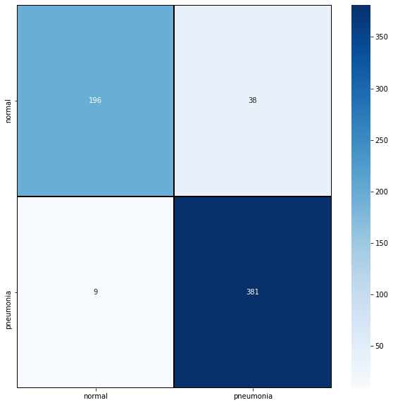
As well as a confusion matrix, which can be visualized with Seaborn. If you're unsure as to what this is, check out this wiki page.
cm = confusion_matrix(y_test, predictions)

plt.figure(figsize=(10,10))
sns.heatmap(cm, cmap="Blues", linecolor='black',
            linewidth=1, annot=True, fmt='', xticklabels=classes,
            yticklabels=classes)
plt.show()
Keras models are extremely easy to save and load:
model.save('todays-date')
Now that we've saved the model, we can turn our attention to the black box analysis of the model using SHAP's GradientExplainer.
Stay tuned for the next part.
Comments
Loading
No results found