Modeling Data with NumPy: Images
NumPy is one of the most important packages for data science and scientific/numerical computing within Python. It provides the foundation of core data science libraries such as Torch, OpenCV, XGBoost, SciKit-Learn, Pandas, and SciPy.
Though we often interface with NumPy through the use of other tools -- such as Pandas, OpenCV, or Torch -- it is good to understand how to work with it directly. Understanding how NumPy is used to model data -- images, audio, video, or tabulated numerical values -- allows you to make informed decisions about how you might process that information using machine learning or other tools. If you are unfamiliar with the term, data modeling refers to how you structure information within a program to accomplish a certain goal.
In this article, we'll take a look at NumPy and how it can be used to work with images. A Jupyter Notebook containing the code in the article can be downloaded here. A Docker environment with NumPy, Pandas, and other dependencies needed can be be found here.
NumPy Fundamentals
NumPy provides an implementation of a data structure called an N-Dimensional array. An array is an ordered collection of values of the same type. N-dimensional means that the array can have any number of dimensions.
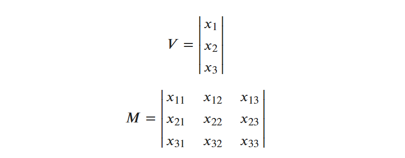
- n-dimensional arrays can be used to model important structures in math like vectors and matrices
- One-dimensional arrays are called vectors and represent a sequence of values. The sequence of values in a vector are often related in some way. They might represent variables describing a single object or event, or they might have some other relationship such as being part of a time-series.
- Two-dimensional arrays are called matrices (or tables) and are comprised of rows and columns. A row or column from a matrix can be treated as a vector. Matrices are very flexible data structures that can be used to represent nearly any type of two-dimensional information, from tabulated structural data such as might be kept in a database to images. Additional detail about how image data is structured can be found below.
- Three-dimensional arrays are comprised of "layers" of two-dimensional arrays and can be used to model a huge variety of two-dimensional data. For example, color images are composed of three stacked "channels" of two-dimensional data. Medical images, comprised of two-dimensional "slices" are often stacked to create volumes. Weather forecasters often use layers of tabulated reports from different locations and use the layers to represent time.
- A dimension refers to the number points needed to retrieve a piece of data (an element) from the array. This number is called a "positional index" and specifies how far from the beginning a piece of data is stored.
- A piece of data can be accessed from a specific location in the array using the index. As data increases in dimensions, the number of indexes required to access the data also increases.
- For one-dimensional data, accessing an element requires the zero-indexed position of the data.
Example array:a = array([0, 1, 2, 3, 4, 5])
Retrieve third element:e3 = a[2] - For two-dimensional data, accessing the data requires two index numbers; one for the row and a second for the column.
Example array:a = array([[0, 1, 2, 3, 4, 5], [6, 7, 8, 9, 10]])Retrieve second element from second row:e22 = a[1,1] - Three dimensional structures require the layer index.
Retrieve second element from second row in the second layer:e222 = a[1,1,1] - Reminder: elements are zero-indexed, which means that the index is always one minus the position.
- For one-dimensional data, accessing an element requires the zero-indexed position of the data.
- A piece of data can be accessed from a specific location in the array using the index. As data increases in dimensions, the number of indexes required to access the data also increases.
High-Performance Computing
NumPy implements the core constructs in C, which makes them very efficient for computation. This is in contrast to most Python data types which are implemented as objects. Objects are easier to work with but require more time and memory for computation, whereas data primitives are not as convenient, but can be manipulated (often in parallel) easily.
Import Dependencies and Supporting Libraries
The code block below imports NumPy and the helper utilities which will be used in this notebook.
- By convention,
numpyis imported under thenpalias. requestsis a library that provides an HTTP transport client. It is useful for fetching data from the web.BytesIOis used alongsiderequeststo provide a "file-like objects" interface. File-like objects are the default interface that Python uses to handle input/output (IO) operations.OrderedDictis used to provide structures for managing the visualization later in the notebook.seaborn(imported under thesnsalias) is used for creating histograms whilematplotlibis used to create a "panel" visualization.
# Helper structueres for working with the image data
from collections import OrderedDict

# Helpers for working with streams
# * requests is an http client for retrieving data
# * BytesIO provides a file-like object that can be provided to methods
#   expecting a file handle.
import requests
from io import BytesIO

# NumPy and plotting tools
import numpy as np
import seaborn as sns
import matplotlib as plt
Creating Arrays
NumPy arrays are created by providing iterable sequences of numbers. The examples in the listing below show how to create a vector (one-dimensional array) and a matrix (two-dimensional array) from a tuple (immutable array) and a nested list of lists. As noted above, NumPy arrays can be any number of dimensions.
# Creating vector and arrays in Python

# Example 1: Vector (1-dimenion)
v = np.array((1, 0, 1))

# Example 2: Matrix (2-dimenions)
m = np.array([
        [2, 3, 5],
        [7, 1, 6],
        [9, 10, 15]])
In addition to creating arrays from Python iterables, NumPy includes a set of methods that can be used to generate arrays directly. These include:
np.arange(upper_limit): returns a one-dimensional array with values ranging from zero to the specified upper limit (the upper value is "exclusive," which means that the range will not include the upper bound)arangeprovides an alternative constructor that can be used to specify the lower bound of the array.- Example:
numpy.arange(2, 10)will producearray([2, 3, 4, 5, 6, 7, 8, 9])
- Example:
- There is also a "step" option that can be included, which controls how large the difference between the values should be. The default value is 1.
- Example:
numpy.arange(2, 10, step=2)will producearray([2, 4, 6, 8])
- Example:
np.zeros(shape): returns an array with provided "shape," filled with zeros. Zeros are useful for creating a placeholder array that will be filled with values as part of some type of computation.shapeis a tuple describing the dimensions of the array.np.zeros((2, 5))would be used for a two-dimensional array with two rows and five columns, for example.
# Example 3: Create an array with a range of values from 0 to
# 1000, stepping by 2.
e3 = np.arange(0, 1000, step=2)


# Example 4: Create an Empty (zero) Three Dimensional Matrix
# with 400 rows, 400 columns, and 3 layers. This structure
# might be used to represent a color image that is 400
# by 400 pixels.
e4 = np.zeros(400, 400, 3)
Shaping Arrays
numpy arrays include a set of properties that describe the number of dimensions, size, and shape of the array.
shapeis a property that contains a tuple describing the number and size of the array- A three-dimensional array similar to
e4above, would return a three-member tuple:e4.shapewould return(400, 400, 3)signifying that the array contains 400 rows, 400 columns, and 3 layers.
- A three-dimensional array similar to
ndimcontains the number of dimensions of the array- Equivalent to calculating the length of
shape:a.ndims == len(a.shape)
- Equivalent to calculating the length of
- The total number of elements in the array can be accessed using the
sizeproperty. This includes all elements across all of the dimensions.- Equivalent to multiplying all of the elements of
shapetogether:a.size == reduce(lambda l,r: l*r, a.shape)
- Equivalent to multiplying all of the elements of
from functools import reduce

# Shape is the core property describing the size of the array.
# It is a tuple describing the size of all of the dimenions.
# For a three dimensional array, it would have three elements:
# * number of rows
# * number of columns
# * number of layers

# Convenience functions are available on the array that
# describe the number of dimensions and the total number of elements.
# These can also be calculated from the shape.

# ndim is the number of dimensions, equivalent to the length of shape
assert e4.ndim == len(e4.shape)

# size is the total number of elements, requivalent to multiplying

assert e4.size == reduce(lambda l,r: l*r , e4.shape)
Reshaping Arrays
One common need in working with data is to take an array that is being modeled in one format and change it to another. For example, a common need in image processing is to calculate the distribution (histogram) for pixel values. While this can be done using a two-dimensional array, it requires additional work that makes the process more difficult. For that reason, a common approach is to "reshape" the two-dimensional image data into a vector. This involves taking each row of data and stacking them end to end. For an 8x8 image, this would mean that you end up with a vector of 64 elements.
NumPy includes a set of methods that can be used to modify the structure of an array. These include reshape and flatten:
a.reshape(shape): modify the structure of the array so that it matches the provided shape.- Example 5, flatten a two-dimensional table to a single dimension, with all rows stacked adjacent to one another:
a.reshape((1, -1)). The 1 in the first dimension of the desired shape refers to a single row. The -1 tells NumPy to calculate the needed number of columns in the array based on the row-size of the original array. - Example 6, create a two-dimensional structure from a one-dimensional array:
np.arange(0, 12).shape((3, 4))The example code first creates a range from 0 to 12, and then reshapes that to three rows and four columns.
- Example 5, flatten a two-dimensional table to a single dimension, with all rows stacked adjacent to one another:
a.flatten(order='C'): create a copy of the array collapsed to a single dimension. Special case ofreshape.- Example 7, flatten an image to a single dimension:
a.flatten(). Equivalent toa.resape((1, -1)).
- Example 7, flatten an image to a single dimension:
# Example 5.11: Flatten a three-dimensional structure to one dimension.
# The -1 tells NumPy determine the number of columns needed automatically.
e51 = e4.reshape((-1,))

# Example 5.2: Restore the original three-dimensional structure.
e52 = e51.reshape((400, 400, -1))

# Example 6: Create a two-dimensional structure from a one-dimensional array
e6 = np.arange(0, 12).reshape((3, 4))

# Example 7: Flatten an array
e7 = e4.flatten()
assert e51.shape == e7.shape
Computation Included
In addition to the core ndarray data type, NumPy also provides efficient implementations of low-level mathematical operations on the data.
# Example 4: Scale a Vector
e2 = v*3

# Example 5: Linear Algegra Dot Product
e3 = m.dot(v)
Modeling Data with NumPy
As noted above, because of the concise way that data can be represented in NumPy, it forms the foundation of many types of numerical computing. Examples include:
- Images
- Tabulated Data
- Video
- Audio
In the remainder of this article, we will focus exclusively on images. Future articles will look at tabulated data, audio, and video.
Images
Images are represented as a set of values organized into a table.
- The table will have a set of dimensions corresponding to its height and width.
- For black and white images, the value of the particular "cell" is the color of the image. 0 for black and a value like 255 (corresponding to the max value of an 8-bit integer) for white.
- For color images, there is more than one table. Each table is called a "channel".
- For images taken with a regular camera (visible light), there are three channels corresponding to red (r), green (g), and blue (b).
- Images are encoded in a "format."
- There are many libraries that can be used to read an image and render it to a NumPy array.
imageiois one library that is used commonly with NumPy.
In the remainder of this section, we will look at how you can utilize NumPy and imageio to work with images. The code shows how to:
- Download images from a remote source using
requestsand BytesIO - Encode the image data to a NumPy array using
imageio - Decompose the image into each of its constituent channels and re-shape the two-dimensional table into a vector that can be used for basic image processing operations, such as creating histograms of pixel intensities.
- Utilize
matplotliband Seaborn to visualize the histograms alongside a visualization of the image
Configure Notebook for Visualization
import imageio # ImageIO handles loading of image data,
from matplotlib.pyplot import imshow as plt_imshow

import IPython, PIL
# When working in a Jupyter notebook, PIL is often used to allow for
# display and visualization of the image at points in a processing
# pipeline

CHANNEL_LABELS = OrderedDict((
    ('r', 'red'),
    ('g', 'green'),
    ('b', 'blue')
))

%matplotlib inline
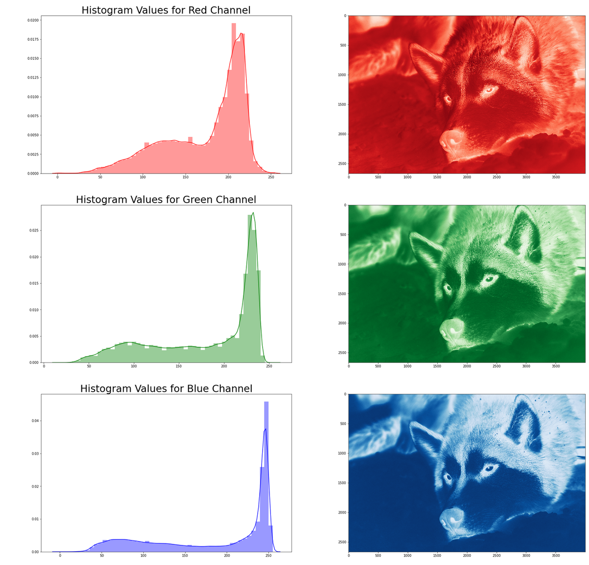
Example Image 1: Wolf in the Snow
The example code below shows the workflow for retrieving an image and using imageio to generate a NumPy array with the pixel data.
requests.getfetches the image from the sourceBytesIOis used to create a file-like object which can be read and processed byimageio.imread
# Example 1: Retrieve an image from a remote
# website and create an array.
# Light colored image.

# Retrieve
r_img_e1 = requests.get(
    "https://oak-tree.tech/documents/115/resnet.wolf.jpg")
img_e1_arr = imageio.imread(BytesIO(r_img_e1.content))

# Check the dimensions of the image
type(img_e1_arr), img_e1_arr.shape
Loading and working with images:
- BytesIO provides an interface for working with remote data
- In Python, nearly all file input/output happens through a "file-like" object
- Requests allow for the fetch of remote data
- The "content" of the request is used to create a stream, which is then read by ImageIO to create an array object.
- The array that is created by ImageIO is 2668 pixels by 4000 pixels with three channels (RGB)
The code in the listing below will display the image inline within a Jupyter Notebook.
# Example 1: Display the image data
IPython.display.display(PIL.Image.fromarray(img_e1_arr))

When working with images, we often care a great deal about the distribution of light and dark values. These are often called the histograms. Breaking images apart by their respective channels and looking at the relative intensity of the histograms for green, or blue, or reg can provide information about where the image may have been acquired. An image that has a large number of intense green pixels might be from a forest, while a red image might indicate a desert, or blue pixels a snowfield.
The code in the example below shows how to:
- Decompose the image into its channel components.
- An array called
cdata1is created by iterating through the layers of image data. - On each pass, all of the pixels from the rows and columns dimensions are collected and "flattened" into a vector.
- The vectors are then aggregated and used to generate a new array.
- An array called
- Generate a histogram of each channel
- The individual rows of the array
cdatagenerated above are fed to Seaborn'sdistplotmethod, which generates the histogram.
- The individual rows of the array
- Plot each histogram and the channel component into a figure
subplotfrommatplotlib.pyplotprovides a way to create panels and fill them with charts like the histogram or imageimshowis used to plot the image data with a specific color encoding
# Example 1: Calculate histograms from the NumPy arrays

# Step 1.1: Re-shape the two-dimensional table for each channel to a vector
# and add the data to the flattened array from above
cdata1 = np.array(
    [img_e1_arr[:,:,i].flatten() for i in range(0, img_e1_arr.shape[2])])

# Step 1.2: Visualize and plot the distributions of pixel data

# Step 1.2.1: Create an output figure for the histograms
plt.pyplot.figure(figsize=(30, 30))

for i, (ccode, clabel) in enumerate(CHANNEL_LABELS.items()):

    # Step 1.2.2: Plot image channel histogram
    plt.pyplot.subplot(3, 2, i*2+1)
    plt.pyplot.title(
        "Histogram Values for %s Channel" % clabel.title(),
        fontsize=30)
    sns.distplot(cdata1[:][i], color=ccode)

    # Step 1.2.3: Plot image channel data
    sub = plt.pyplot.subplot(3, 2, i*2+2)
    sub.imshow(img_e1_arr[:,:,i],
        interpolation='nearest', cmap='%ss' % clabel.title())
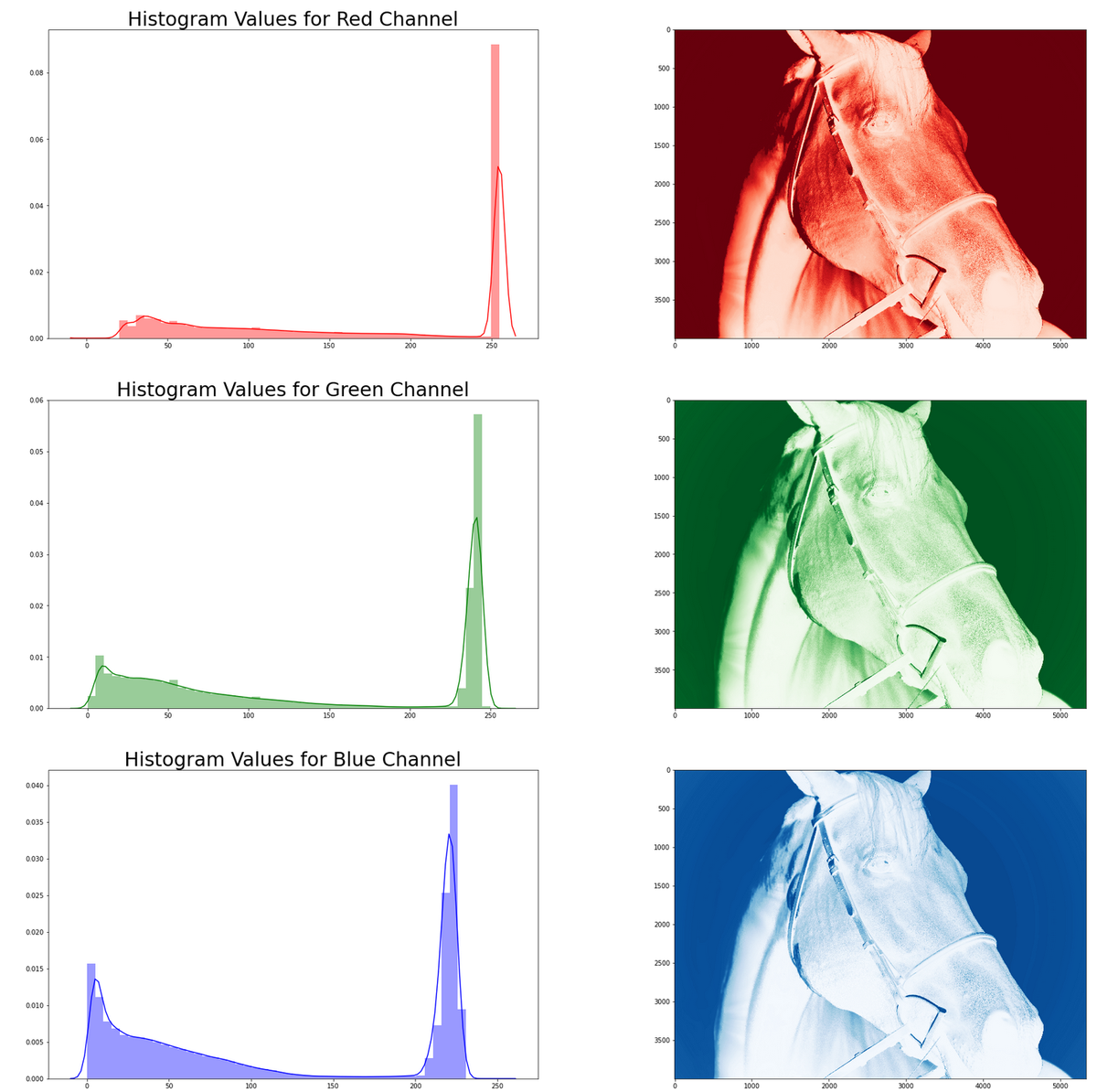
Example 2: Horse
This second example provides a contrast to the image above. The same procedure to fetch and display the image is used as is the procedure for decomposing the channels and plotting the histograms.
# Example 2: Dark Colored Image
r_img_e2 = requests.get(
    'https://oak-tree.tech/documents/117/resnet.horse-bridle.jpg')
img_e2_arr = imageio.imread(BytesIO(r_img_e2.content))

# Display the image
IPython.display.display(PIL.Image.fromarray(img_e2_arr))

# Step 2.1: Segment the pixel data by channel
cdata2 = np.array(
    [img_e2_arr[:,:,i].flatten() for i in range(0, img_e2_arr.shape[2])])

# Step 2.2: Visualize and plot the distributions of pixel data

# Step 2.2.1: Create an output figure for the histograms
plt.pyplot.figure(figsize=(30, 30))

for i, (ccode, clabel) in enumerate(CHANNEL_LABELS.items()):

    # Step 2.2.2: Plot image channel histogram
    plt.pyplot.subplot(3, 2, i*2+1)
    plt.pyplot.title(
        "Histogram Values for %s Channel" % clabel.title(),
        fontsize=30)
    sns.distplot(cdata2[:][i], color=ccode)

    # Step 2.2.3: Plot image channel data
    sub = plt.pyplot.subplot(3, 2, i*2+2)
    sub.imshow(img_e2_arr[:,:,i],
        interpolation='nearest', cmap='%ss' % clabel.title())
Comments
Loading
No results found