First Steps With Jupyter
Jupyter is an open-source project that provides an interactive development environment that has become popular with Data Scientists, Data Engineers, software developers, and analysts. Jupyter runs special documents (called notebooks) which integrate code, documentation, equations, and other information into a single page. Such notebooks -- because they can be used to fully describe all of the steps of an analysis or workflow along with code, visualizations, and data -- have become the defacto standard for Data Science and Engineering development.
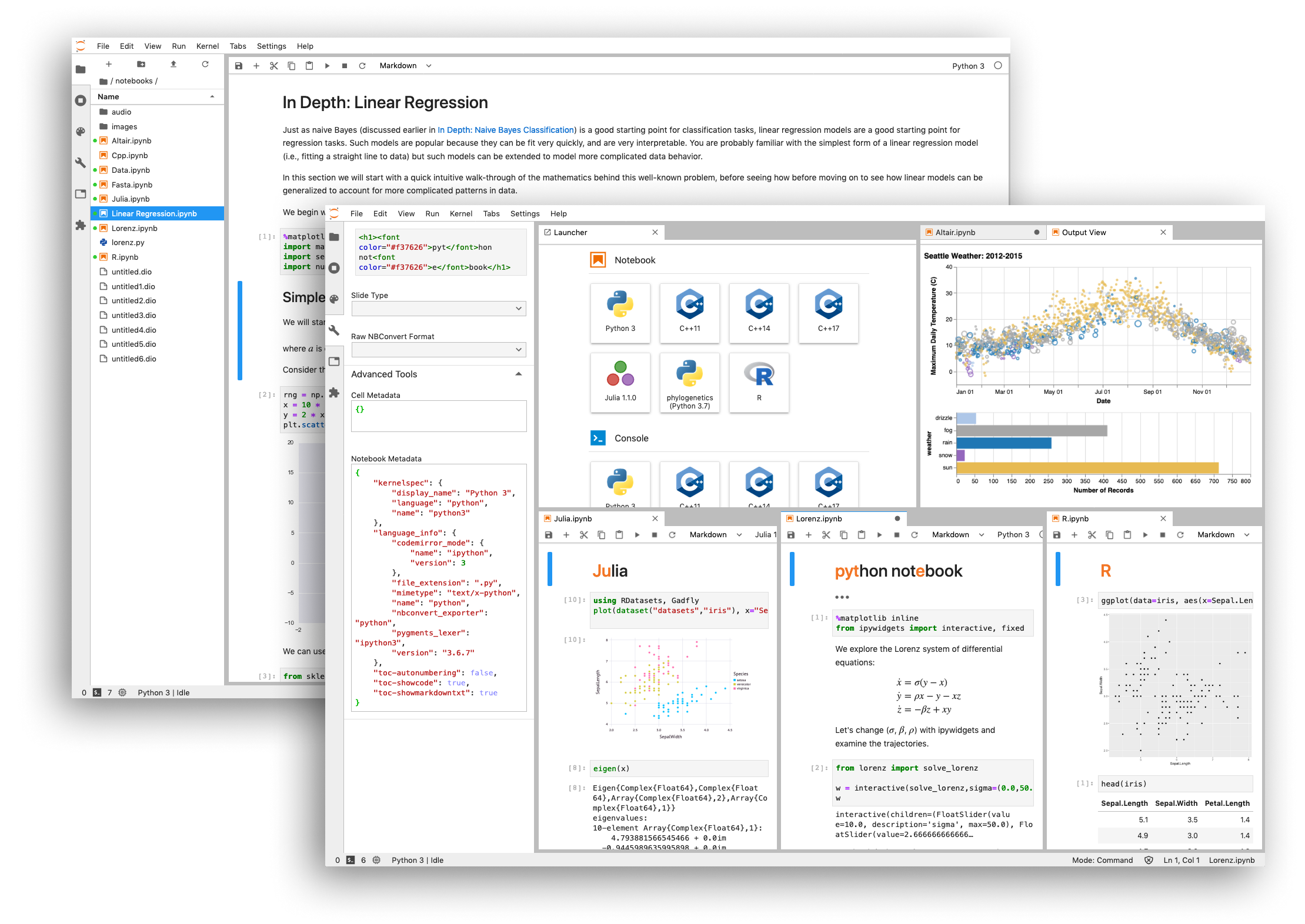
JupyterLab is the current iteration of the Jupyter interface. It provides a robust IDE which allows users to work with multiple notebooks simultaneously, view the results and associated data, run supporting commands in programming terminals, or access the shell of the environment where the IDE is running. The environment is configurable, which allows for users to have a custom workspace that is flexible to their development needs.
This tutorial introduces Jupyter, its features, and some of the types of tasks that it allows.
The Jupyter Project
Jupyter started as "iPython," an interactive environment to extend the default Python interpreter with additional features to help facilitate scientific computing. Robert Kern and Fernando Pérez, two of the early Jupyter developers, wanted to create an environment which could be used to display images and graphs inline, and might serve as the basis of a "literate programming" model for Python (similar to Mathematica or Maple notebooks). After having success with an initial prototype, other developers expressed interest in creating "kernels" for programming languages other than Python.
In response to that interest, in 2014, Jupyter was split from iPython to make it easier to create alternative Kernels. The developers decided to make the architecture modular with a frontend piece and a pluggable backend. Since then, the frontend pieces and the interface have been managed by the Jupyter team, while the default Python kernel continues to be called iPython and is developed in parallel.
While initially focused on the development of kernels and notebooks, the Jupyter project has continued to evolve and has become an entire suite of tools to facilitate interactive computing.
- The core of these efforts is, of course, the Juptyer Notebook itself. As noted above, notebooks are an interactive computational environment allowing for rich text (rendered from Markdown), mathematics, plots and media. Notebooks are implemented as a "runtime" which includes a local component (where code is entered and results displayed) and a remote server (called a kernel) where the logic is executed.
- Notebooks package their code and associated information in a JSON file with an .
ipynbextension. - The Jupyter project has created a full specification describing Notebooks and their associated components. Because the format is open, there have been several different runtimes implemented, with the most popular being the Jupyter web application. Alternatives are also available, however, such as the Jupyter Qt Console.
- Notebooks package their code and associated information in a JSON file with an .
- JupyterLab, also as explained above, is a broad set of additions to the web application intended to make Jupyter a powerful tool for data driven development.
- JuptyerHub: a management application designed to securely host Jupyter instances for many users providing authentication, proxy, and persistence.
Install and Run Jupyter
Jupyter can be downloaded and deployed from a number of locations. If you wish to be up and running quickly, it is possible to use pre-packaged environments such as the Oak-Tree Big Data Lab (which uses Docker) or one of the images provided by Jupyter Stacks.
If you wish to download and install it on your own computer (perhaps using of a virtual environment, though that is optional), it is available through both pip and Anaconda. The instructions below show how to install via pip.
# Install Jupyter locally
pip install jupyter

# Start the Jupyter Environment
jupyter lab
The commands in the listing start JupyterLab. If you wish to run the "classic" notebook interface, that can be started by running jupyter notebook.
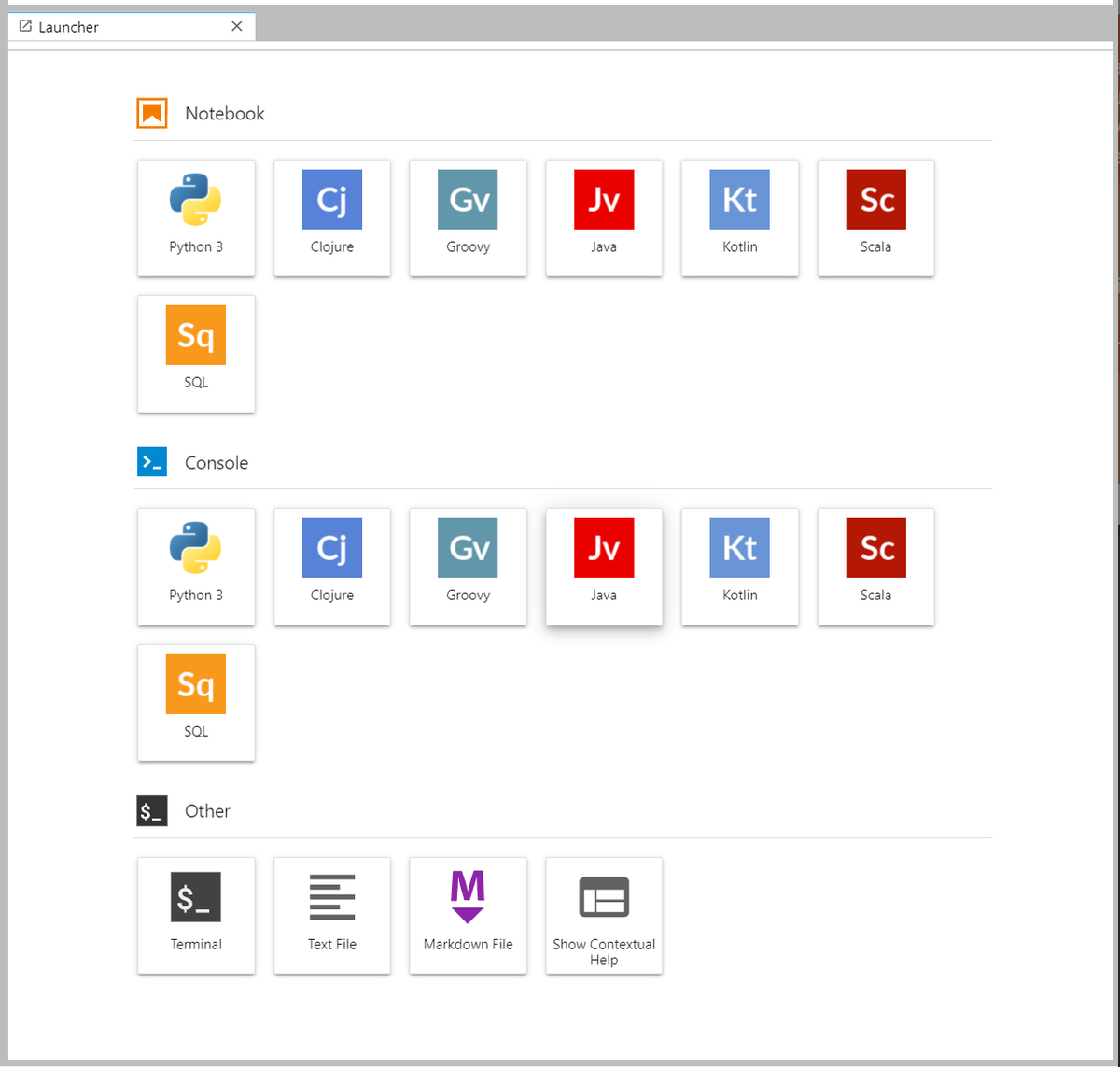
Once the server is running, you will see a "launcher" that allows you to select the type of resource you would like to open. Jupyter Lab provides three classes of resources: notebooks, terminals, and others (which include things like text/markdown documents and system shells). To start a kernel and begin using the system, select one of the resource types.
The De-Facto Standard for Data Science
Because of its interactivity and rich-media support, Juptyer Notebooks have come to dominate the tools used for exploratory data analysis and machine learning development. They allow for text and code to live side-by-side, providing an ideal model for documenting data structure and the choices that led to a conclusion or a machine learning model.
One of the reasons for their success is that Jupyter Notebooks are extremely simple. They are a collection of "cells" that contain content. Content may be one of three types:
- Code: Logic which should be sent to the kernel and executed as a block.
- Output: Data results sent back from the kernel and displayed, either as direct output, or as an interactive "widget."
- Markdown or LaTeX text
A notebook can be run as a traditional program, which is to say, means that you start at the beginning and run all of the code until you reach the end. But it's real value comes in processes that require exploration and iterative prototyping such as Machine Learning Model development and Exploratory Data Analysis.
Creating Cells and Executing Code
When a notebook loads, you will see an input cell. The cell should be highlighted and have a blue border. If you click on the input and begin typing, the color of the border will change to green. Jupyter notebooks have two different keyboard input modes, the state of which is indicated by the color of the cell.
- Edit Mode allows you to type code or markdown into the cell and submit the code to the kernel and is indicated by a green border.
- Command Mode allows you issue notebook level commands (such as adding or removing cells) and is indicated by a blue border.
Commands can be executed by entering Shift+Enter or by clicking on the "Run" button in the toolbar.
Accessing Documentation and Contextual Help
The Jupyter environment supports tab completion and includes contextual help. Help for commands can be accessed by using the ? operator. For example, if you wished to retrieve additional information about functions in the math package:
import math
math.p?
Multicursor Support
Jupyter supports multiple cursors, similar to Sublime Text or Vim. To access the feature, click and drag your mouse holding Alt.
Exploratory Data Analysis
One of the difficult realities of working with data is that there usually isn't a straightforward process to distill the raw information into insight. Stephen Few expresses this succinctly:
We live in a data-rich world ... [but] most of us stand on the shore of a vast sea of available data, suited up in the latest diving gear and equipped with the latest tools and gadgets, with hardly a clue what to do ... The problem is that [we] don't know how to dive into the sea of information, net the best of it, bring it back to shore, and sort it out.
What Few describes is the process of exploratory data analysis: taking the information and using summaries and visualizations to start to make sense of it, and then deciding on more formal procedures to draw rigorous conclusions. Jupyter integrates with the broader ecosystem of both Python (Pandas, SciKit-Learn, Seaborn, TensorFlow, PyTorch, and more) and other tools to allow you to summarize and visualize data.
Because exploratory data analysis is messy, working in a Jupyter notebook allows for variations of different procedures while providing a complete log of the code and work product that produced a particular result. When combined with the notes about why specific decisions were made, this provides a way to communicate notes to colleagues and the broader public.
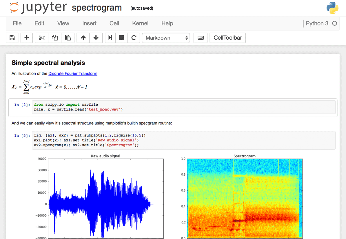
The figures below show examples of the types of visualizations that can be created inside of Jupyter and the code used to generate them.
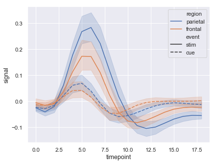
import seaborn as sns
sns.set(style="darkgrid")

# Load an example dataset with long-form data
fmri = sns.load_dataset("fmri")

# Plot the responses for different events and regions
sns.lineplot(x="timepoint", y="signal",
    hue="region", style="event",
    data=fmri)
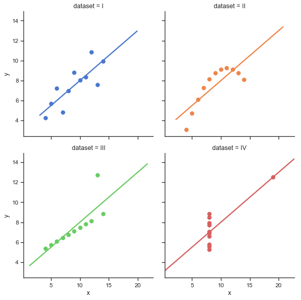
import seaborn as sns
sns.set(style="ticks")

# Load the example dataset for Anscombe's quartet
df = sns.load_dataset("anscombe")

# Show the results of a linear regression within each dataset
sns.lmplot(x="x", y="y", col="dataset", hue="dataset", data=df,
    col_wrap=2, ci=None, palette="muted", height=4,
    scatter_kws={"s": 50, "alpha": 1})
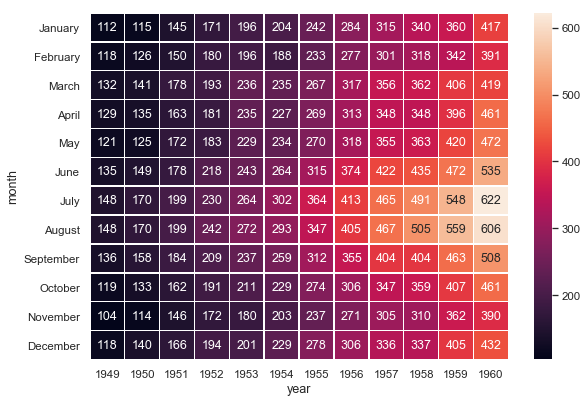
import matplotlib.pyplot as plt
import seaborn as sns
sns.set()

# Load the example flights dataset and conver to long-form
flights_long = sns.load_dataset("flights")
flights = flights_long.pivot("month", "year", "passengers")

# Draw a heatmap with the numeric values in each cell
f, ax = plt.subplots(figsize=(9, 6))
sns.heatmap(flights, annot=True, fmt="d", linewidths=.5, ax=ax)
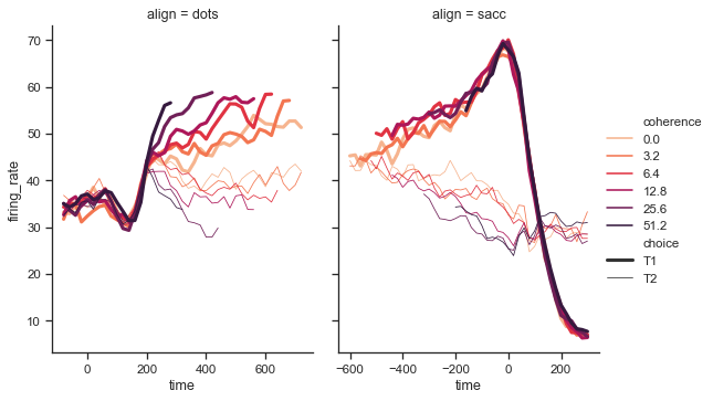
import seaborn as sns
sns.set(style="ticks")

dots = sns.load_dataset("dots")

# Define a palette to ensure that colors will be
# shared across the facets
palette = dict(zip(dots.coherence.unique(),
                   sns.color_palette("rocket_r", 6)))

# Plot the lines on two facets
sns.relplot(x="time", y="firing_rate",
    hue="coherence", size="choice", col="align",
    size_order=["T1", "T2"], palette=palette,
    height=5, aspect=.75, facet_kws=dict(sharex=False),
    kind="line", legend="full", data=dots)
Machine Learning Model Development
Like exploratory data analysis, training and evaluating machine learning models is a highly iterative process. When creating a machine learning model:
- Data has to be analyzed and visualized to assess for patterns in the data that might be further explored using a machine learning algorithm.
- Specific variables/features of interest need to be identified, their potential relationship to one another assessed (correlation) and new variables created (feature engineering).
- Individual algorithms trialed and choices made about which might produce the best results and what combination of parameters will provide the best accuracy (hyper-parameter tuning).
The wash, rinse, and repeat process benefits greatly from Jupyter's integration with visualization tools and literate programming model. In effect, the notebook becomes a record of the many experiments required to build accurate models. The code below demonstrates a basic procedure for building and assessing a machine learning model: configure the notebook, retrieve a remote file and create a structured dataset, split the data into a training and testing set, train a model, and assess the model's accuracy.
Notebook Setup
With minimal configuration, Jupyter notebooks become powerful visualization tools capable of showing plots inline.
# Data Libraries
import pandas
import numpy as np
import matplotlib

# Machine Learning Libraries
from sklearn.linear_model import LogisticRegression
from sklearn.tree import DecisionTreeClassifier
from sklearn.ensemble import RandomForestClassifier

# Configure notebook for visualization
%matplotlib inline
Load and Prepare Data
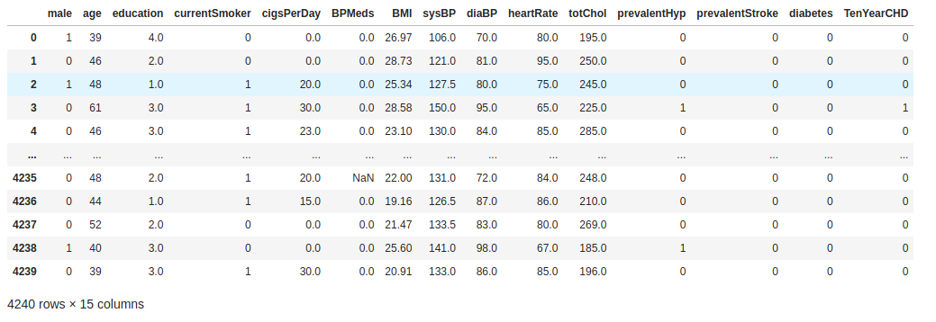
Python has long had a "batteries included" and "simplicity first" mindset. This approach to building systems usually results in interfaces that are powerful and easy to use. Retrieving a file from a remote source with Pandas (the primary library for structured data in Python), for example, is no more complex than providing the URL. From there, Jupyter's enhanced support for the Pandas data frame and other tabular structures allow you to explore and inspect data quickly and efficiently.
# Load data remotely
patientdata = pandas.read_csv(
    'https://oak-tree.tech/documents/96/framingham.csv')
patientdata
While reviewing the data, I noticed that there are some rows with missing values. Those need to be removed form the dataset before creating a model.
# Remove rows with missing values from the dataframe.
# This is only one appraoch to the problem of missing data.
# There are alternative approaches that might be used to fill
# the missing values without skewing the results.
patientdata = patientdata.dropna(axis='columns')
Create Helper Methods
Jupyter notebooks are programs, which means that you can create helper functions to abstract away the details of repetitive processes or to customize a workflow for a specific use-case. The code in the listing below creates methods for creating instances of machine learning algorithms and fitting them to a set of training data.
def train(ModelClass, features, target):
	'''	Train a model using the provided features,
	    target, and model class
	'''
	model = ModelClass()
	model.fit(features, target)
	return model


def predict(model, features):
	'''	Use the provided model to create predictions
	    on the provided features
	'''
	return model.predict(features)
The code in the listing below helps to automate the train/testing split by modifying a data frame to the format expected by SciKit-Learn's API. Given a dataset, it pulls out the outcome variable of interest to a separate structure, removing it from the frame so that it can be used as a set of features. Next, it uses the train_test_split from sklearn.model_selection to segregate the dataset into two groups.
from sklearn.model_selection import train_test_split


def ml_split_data(target, df, test_size=0.3):
	'''	Create a train/testing split for the specified target
	    from the provided dataframe

		@input test_size (default=0.3): Size of the set
		which should be used for testing
			the model.
	'''
	# Pull target into a series, drop the target from the data frame
	y = df[target]
	X = df.drop(columns=target)

	return train_test_split(
	    X, y, test_size=test_size, random_state=42, stratify=y)
Train and Apply Machine Learning Models
Generating a model is a matter of applying the procedure: create the training/testing split, train the model, assess the model.
# Create the Training/Testing Split
X_train, X_test, y_train, y_test = ml_split_data('TenYearCHD', patientdata)

# Train the Model Using the Training Data, Test the Model Using the Testing Data
dtmodel = train(DecisionTreeClassifier, X_train, y_train)
dtmodel.score(X_test, y_test)
The DecisionTreeClassifier model generates predictions that are about 75% accurate.
Assess Alternative Models
SciKit-Learn provides a uniform interface intended to rapidly prototype many different algorithms and make comparisons. RandomForestClassifier is often used as an alternative to decisions trees (it is an example of an "ensemble model").
rfmodel = train(RandomForestClassifier, X_train, y_train)
rfmodel.score(X_test, y_test)
The RendomForestClassifier creates predictions that are about 82% accurate, a significant improvement.
Just Getting Started
Jupyter is a remarkably powerful tool for interactive computing and the examples we've looked at to this point barely scratch the surface of what the platform is capable of.
Big Data Integration
Using plugins, Jupyter is able to work with Big Data tools such as Apache Spark. This makes it possible to analyze and visualize the same data with Pandas, SciKit-Learn, ggplot2, and other data analytics tools.
Interactive Output
Once results have been finalized, Jupyter allows you to export to a huge number of formats which support rich, interactive output. HTML, images, videos, LaTeX, and custom widgets can be rendered to PDF, web pages, slides, and interactive dashboards.
Polyglot Programming
While this article has focused on Python, Jupyter supports over forty programming languages including Scala, R, C#, C++, Haskell, and Scala. Many of these languages can be added by integrating the BeakerX extension.
Publish and Share
Notebooks can be quickly shared with others in their native format through the use of email, DropBox, GitHub, GitLab, and the Jupyter Notebook Viewer.
What Next?
Like what you see and ready to take the next steps, check out of some of resources below:
- If interested in the capabilities of the environment and how you can extend it with custom interactive components and widgets, check out this video from SciPy that shows how to create Interactive Widgets within Jupyter.
- For additional information about how Jupyter works with Big Data, check out our guide to Spark on Kubernetes.
- Part 1: How do you get up and running with Spark on a Kubernetes cluster?
- Part 2: After you've got Spark running on Kubernetes, how can you integrate the runtime with Jupyter?
- Part 3: When working with data in the cloud, where should it live and how can you access it from your programs?
- Part 4: The Jupyrer ecosystem is full of tools to extend the capabilities of Jupyter. One of the most popular is BeakerX. What is BeakerX and what additional functionality does it provide to Jupyter?
- Ready to Get Started? Check out the Oak-Tree Data Development Lab, a collection of containers that can be used to work with Jupyter, Kafka, Spark, and object storage (MinIO). Instructions to download and configure the containers are in the linked article and the
gitrepository includes example notebooks of how to work with both machine learning libraries and Spark.
Comments
Loading
No results found